How to Calculate A/B Test Sample Size for Conversion Rates (U.S. Audience)

Whether you run growth experiments for a SaaS product or an e-commerce storefront, you need enough data to detect a meaningful change in conversion. This guide shows you exactly how to size your A/B tests for binary outcomes (converted vs not), use reputable calculators, cross-check with code, and estimate runtime using U.S. traffic patterns.

• Difficulty: Intermediate (you should be comfortable with percentages and basic statistical terms)
• Time to complete: 30–60 minutes for setup and verification
• You’ll walk away with: Clear inputs (baseline rate, MDE, alpha, power, allocation), a computed per-variant sample size, code snippets to validate results, and a realistic duration estimate.

What You Need to Decide First

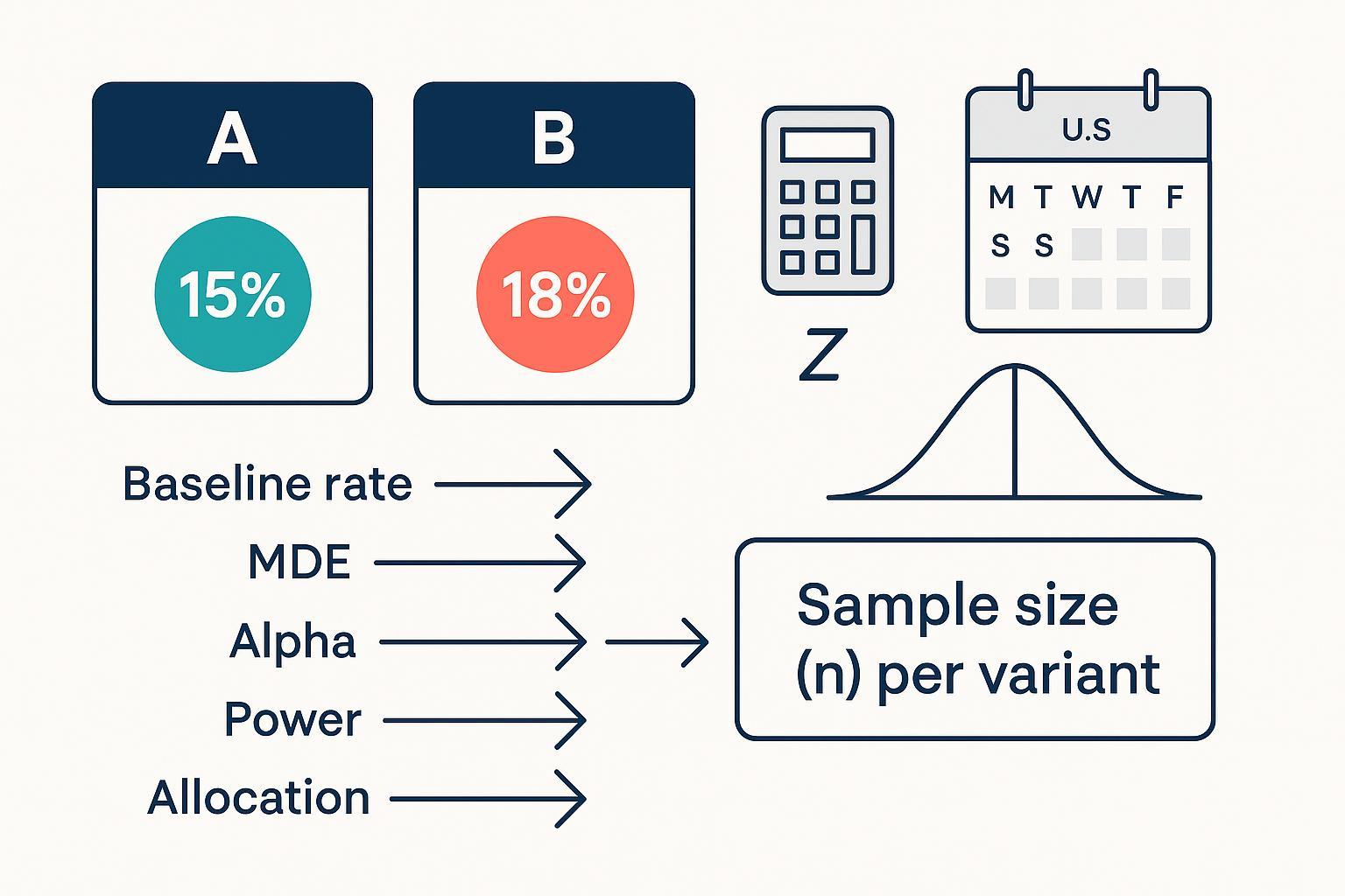
Before you touch a calculator, lock in these inputs. Being explicit prevents underpowered tests and deadline-driven tweaks.

• Baseline conversion rate (p1): Use recent, representative data. If your business is seasonally sensitive, avoid windows skewed by U.S. holidays unless you are designing for that period (e.g., Black Friday/Cyber Monday). I usually pick the past 2–4 weeks excluding major promotions.
• Minimum Detectable Effect (MDE): Define the smallest change that is worth acting on. Express both absolute and relative. Example: from 2.0% to 2.5% is +0.5 percentage points and +25% relative. Smaller MDE requires larger samples.
• Significance level (alpha, α): Common default is 0.05 for two-sided tests.
• Power (1 − β): 0.80 is typical; 0.90 if you want stronger sensitivity.
• Allocation ratio: 1:1 is most efficient. If you need 1:k for rollout or ethics, expect a larger total N.
• Directionality: Two-sided unless you have a justified directional hypothesis. One-sided needs smaller N at the same power but should be pre-declared.

The Statistical Backbone (Plain-English)

A/B tests on conversion rates compare two proportions. Under the null (no difference), we use a pooled estimate of the conversion rate to build the test statistic. When sample sizes are adequate, the difference in sample proportions is approximately normal.

• Pooled proportion under H0: p̂ = (x1 + x2) / (n1 + n2)
• Pooled standard error: SEpooled = sqrt( p̂(1 − p̂)(1/n1 + 1/n2) )
• Z statistic: Z = (p̂1 − p̂2) / SEpooled

For confidence intervals, you use the unpooled standard error: SE = sqrt( p̂1(1 − p̂1)/n1 + p̂2(1 − p̂2)/n2 ). These definitions and conditions for the normal approximation are covered in accessible texts such as the Difference of Two Proportions chapters in OpenIntro via LibreTexts and Penn State’s STAT notes. See, for example, the overview in OpenIntro’s section on the difference of two proportions (LibreTexts, 2025)./06:_Inference_for_Categorical_Data/6.02:_Difference_of_Two_Proportions) and the pooled SE setup in Penn State STAT 415: Comparing Two Proportions.

A practical sample size approximation for equal allocation (n1 = n2 = n) and two-sided tests to detect Δ = p2 − p1 uses a blend of variance terms under H0 and H1:

n ≈ [ z1−α/2 · sqrt(2 p̄(1 − p̄)) + z1−β · sqrt( p1(1 − p1) + p2(1 − p2) ) ]² / Δ², where p̄ = (p1 + p2)/2.

In practice, most teams rely on validated software to compute n directly and handle edge cases; we’ll use R and Python below and cross-check with reputable calculators.

Step-by-Step: Size Your Test and Estimate Duration

Step 1: Gather a Representative Baseline and Traffic Snapshot

• Pull the baseline conversion rate from a stable window. For U.S. consumer businesses, check weekday/weekend differences and avoid windows distorted by major holidays unless you are testing for that period.
• Note daily eligible traffic and the expected percentage of visitors who can see the test. This will be used to convert sample size into calendar days.

Verification: Confirm the baseline sample has adequate events (rule-of-thumb: expected successes and failures per arm ≥ 10 at your planned sample size). This supports the normal approximation discussed in the OpenIntro materials linked above.

Step 2: Choose Your MDE and Translate Between Absolute and Relative

• Tie MDE to business value. If +0.5 pp at a 2.0% baseline unlocks material revenue, keep it. If timelines are tight, consider whether a larger MDE is acceptable.
• Convert formats: Absolute Δ (pp) = target − baseline. Relative change = Δ / baseline.

Tip: I usually sanity-check MDE against historical uplift from similar changes to avoid wishful thinking.

Step 3: Set Alpha, Power, Allocation, and Direction

• Defaults: α=0.05 (two-sided), power=0.80, allocation=1:1.
• One-sided vs two-sided: Only use one-sided if an opposite-direction effect would not change your decision. One-sided uses z1−α (e.g., 1.645 at α=0.05) instead of z1−α/2 and reduces n.
• Unequal allocation: If you set 1:k (e.g., 1:3) to limit exposure, expect total N to increase for the same power.

Step 4: Compute Sample Size with a Calculator (and See the Trade-offs)

Use at least one transparent calculator, then cross-check with code.

• Evan Miller’s A/B test sample size calculator is explicit about inputs and outputs: Evan Miller’s sample size calculator. Enter baseline p1, target p2 (or Δ), α, power, and allocation. It assumes independent Bernoulli trials and uses standard normal approximations.
• Optimizely’s practical guidance explains how to translate sample size into test duration and common inputs: see Optimizely’s “How to calculate sample size of A/B tests” (blog, 2019).
• If you prefer platform-style inputs, compare with Amplitude’s Sample Size Calculator; it takes baseline rate, MDE, and confidence level.

Worked example (numbers illustrative):

• Baseline p1 = 0.020 (2.0%)
• Target p2 = 0.025 (2.5%), so Δ = 0.005 (absolute) = +25% relative
• α = 0.05 (two-sided), power = 0.80, allocation = 1:1

Input these values and record the per-arm n. Then proceed to code to validate.

Step 5: Cross-Check with Code (R and Python)

R (equal allocation):

# Detect 2.0% vs 2.5%, alpha=0.05, power=0.80
power.prop.test(p1 = 0.02, p2 = 0.025, sig.level = 0.05, power = 0.80, alternative = "two.sided")

R (unequal allocation supported via pwr):

# Effect size h for two proportions
library(pwr)
h <- ES.h(0.02, 0.025)
# Solve for n1 and n2 with ratio, two-sided
a <- pwr.2p2n.test(h = h, n1 = NULL, n2 = NULL, sig.level = 0.05, power = 0.80, alternative = "two.sided")
a

The R help for power.prop.test documents parameters and behavior; see the official manual page: R base stats: power.prop.test (manual). For unequal sizes, the pwr package offers pwr.2p2n.test and the ES.h helper; see pwr package documentation (Rdocumentation).

Python (statsmodels):

from statsmodels.stats.proportion import samplesize_proportions_2indep
# two-sided, ratio=1 means 1:1 allocation
n1 = samplesize_proportions_2indep(diff=0.005, prop2=0.02, alpha=0.05, power=0.80, ratio=1, alternative='two-sided')
print(n1)  # per-arm sample size

Statsmodels documents these functions and parameters; see statsmodels: samplesize_proportions_2indep (stable docs).

Verification: The calculator and code should agree within rounding differences. If they don’t, check tails (one vs two-sided), allocation ratio, and whether you used absolute vs relative MDE.

Step 6: Translate Sample Size into U.S.-Aware Duration

• Total required N = n1 + n2. With ratio r = n2/n1, N = n1 + r·n1.
• Duration (days) ≈ N / average daily eligible traffic. Adjust for day-of-week seasonality: many U.S. sites see lower conversion on weekends; plan for a representative mix.
• Optimizely provides accessible tips for mapping sample size to runtime, including setting realistic expectations for traffic and conversion variability in practice; see their blog guidance linked above.

Example: If each arm needs 25,000 visitors and you average 10,000 eligible visitors/day, a 1:1 test would take about 5 days at steady traffic. Add buffer for weekends or upcoming holidays.

Step 7: Verification Checklist and Common Error Prevention

• Confirm baseline window is representative (exclude unusual promotions unless intentional).
• Fix MDE, alpha, power, allocation before you compute; don’t tweak post hoc to “fit” a deadline.
• Compute n using two methods (calculator + code) and compare.
• Validate expected successes/failures per arm ≥ 10 at planned n.
• Estimate duration with realistic weekday/weekend mix; re-check if a U.S. holiday arrives mid-test.
• Preplan stopping rules; avoid unplanned peeking.

Troubleshooting and Edge Cases

• Very low baseline rates (<1%): Normal approximation may be weak. Consider exact or simulation-based approaches, or aggregate events into a higher-frequency metric. For an overview of Fisher’s exact test, see LibreTexts: Fisher’s Exact Test/02:_Tests_for_Nominal_Variables/2.07:_Fisher's_Exact_Test).
• Unequal allocation (1:k): Expect larger total N. Use pwr.2p2n.test in R or ratio in statsmodels to compute per-arm sizes precisely.
• One-sided tests: Only when justified a priori; use one-tail critical value z1−α. In statsmodels, set alternative='larger' or use the one-tail function where appropriate; one-sided reduces n relative to two-sided.
• Sequential peeking: Naive interim looks inflate Type I error. If you must monitor, use a preplanned group-sequential framework with alpha spending (e.g., O’Brien–Fleming or Pocock). For a practitioner-oriented comparison, see Spotify Engineering’s 2023 overview of sequential testing frameworks.

A Worked, Business-Realistic Example

Scenario: U.S. DTC brand testing a free-shipping banner.

• Baseline p1 = 3.0% (weekday average over the past 3 weeks; weekends are 2.5%)
• MDE: +0.4 pp (target p2 = 3.4%; +13.3% relative)
• α=0.05, power=0.80, allocation=1:1, two-sided
• Daily eligible traffic: 20,000 visitors (15k weekdays, 10k weekends)

Compute per-arm n via R and Python as above; suppose both return ~38,000 per arm. Total N ≈ 76,000. Duration ≈ 76,000 / average daily eligible traffic. At a blended 17,000/day, expect ~4.5 days; add buffer so you cover a weekend and at least one full weekday cycle.

Notes on Assumptions and When to Adjust

• Independence and stable data-generating process: If the experiment changes traffic composition (e.g., a concurrent ad campaign), your baseline may shift; re-estimate if needed.
• Conversion definition: Be precise about eligibility and event logging; mismatches inflate variance.
• Guardrails: If you track guardrail metrics (e.g., bounce rate), treat them as descriptive unless you designed the test for multiple comparisons and adjusted alpha accordingly.

Resources and Documentation

• Two-proportion inference and pooled SE definitions: see OpenIntro’s “Difference of Two Proportions” (LibreTexts)./06:_Inference_for_Categorical_Data/6.02:_Difference_of_Two_Proportions) and Penn State STAT 415 lesson on comparing two proportions.
• R base stats manual: power.prop.test; R pwr package doc: pwr.2p2n.test and ES.h.
• Python statsmodels: samplesize_proportions_2indep (stable docs).
• Practitioner guidance on mapping sample size to duration: Optimizely’s sample size blog.
• Calculator alternative: Amplitude Sample Size Calculator and Evan Miller’s calculator.

Quick Pre-Launch Checklist

• Baseline window is representative and U.S. seasonality accounted for.
• MDE, α, power, allocation set and documented.
• Sample size computed via calculator and code; results agree.
• Expected successes/failures per arm ≥ 10 at planned n.
• Duration estimated from daily eligible traffic; buffers added for weekends/holidays.
• Stopping rules and peeking policy set; team aligned.

Run your next experiment with confidence: size it correctly, verify the math, and schedule it to fit real U.S. traffic patterns.